How to Strikethrough in Microsoft Excel

Microsoft Excel is one of the most underrated software at your fingertips. You can use it to create a whole lot of content, from simple tables to complex graphs and charts. Yet, many people are intimidated by using Excel because they don’t know where to start.

One way to make your content neater is by applying strikethroughs whenever you want to cross off a task or goal. Let’s look at how to strikethrough in Microsoft Excel using different ways.

Use a Keyboard Shortcut

Typing in shortcuts is the most straightforward way of using strikethrough in Excel. Read them below:

1. To strikethrough text in Excel, use the keyboard shortcut Ctrl+5 ( if you’re using Windows) or Command-5 (if you’re using Mac). You can also use this same command to add a strikethrough to your existing text.
2. After you’ve entered your desired strikethrough, select it again and hit Enter to make it permanent.
3. If you want to remove all of the events from your text (like how you did above), enter Clear followed by Ctrl+A (Windows) or Command-A (Mac).

Use the Format Cells Dialog Box

If you don’t want to use your keyboard all the time or aren’t good at remembering shortcut keys, you can strikethrough texts using the format cells dialog box. Here’s how:

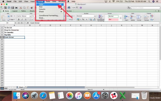
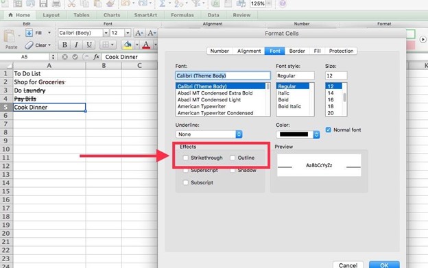
1. First, select the cells you want to format to use strikethrough in Microsoft Excel. Once done, click on the Format Cells dialog box and select strikethrough from the Font menu. You can also choose between multiple colors for each effect by selecting one from the Color dropdown list in this window.

2. When you’re finished making all your selections, click OK to apply your new font settings to all selected cells simultaneously.

Add Strikethrough to Excel’s Quick Access Toolbar

The strikethrough function is usually readily available on the quick access toolbar. But if not, there’s a way you can add it for easy access.

To add a strikethrough command to Excel’s Quick Access Toolbar, you will need to follow these steps:

1. Head to the Quick Access Toolbar and select Customize.
2. Click on More Commands at the bottom of your toolbar. You can also press CTRL+M. Cmd + M if you’re using a Mac.
3. Select Strikethrough, then click on one of two buttons: Add or Remove. It will bring up a dialog box where you can select whether or not you want this tool added permanently.
4. Click OK after making your choice and restart Excel if needed (you can also do this by pressing F5).

Strikethrough Partial Text in Excel

Using a strikethrough is an excellent way to cross off tasks or goals you need to accomplish. That way, you don’t have to delete the text if you want to return to it. But what do you do if you only want to cross off a portion of the text?

Here’s how:

You can use the strikethrough function to cross off a text from a cell. This is useful if you want to delete text in one cell, but not in others, or if you have a column of cells with different types of content and would like to delete only certain parts of that column.

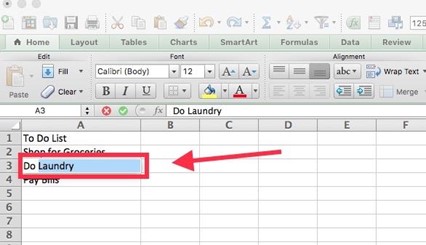
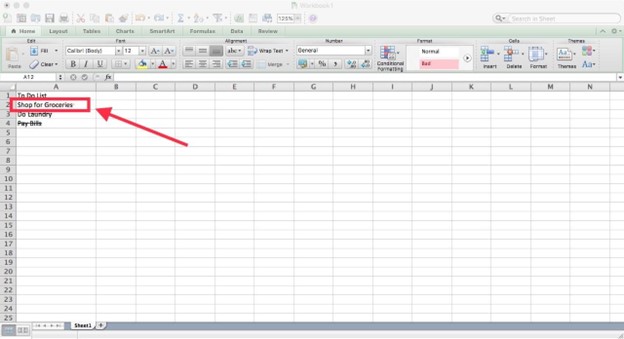
1. To use this feature, highlight the portion of the text you want to put the strikethrough.

2. Open up the Format menu, where Strikethrough is listed as one of many options for formatting your selection. Check strikethrough and uncheck the normal font so that only the highlighted portion will be affected.
3. It is crucial to uncheck the normal font otherwise, the strikethrough will apply to the entire text in the cell.

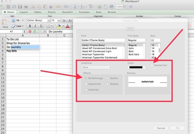
It will look something like this:

Strikethrough Text in Excel With a Different Color

Unfortunately, you can’t change the color of the strikethrough. You can only change the text’s color. To do that:

1. Open the Format menu and check strikethrough. You’ll see there is a separate box indicating the color.
2. Select your preferred color and click ok. Your text should now be in a different color.

You can try a few things if you want a different color strikethrough. Although it does not use the strikethrough function, it does achieve the same effect! The easiest way is to use the shapes function to draw a line resembling a strikethrough. Here’s how you can do this:

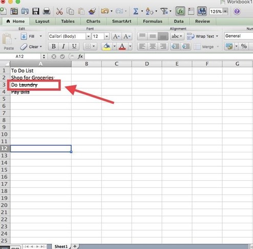
1.Select the cell containing the text you want to apply the strikethrough.
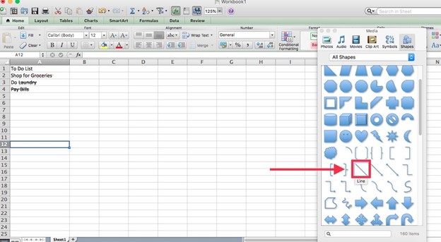
2.Open the shapes tab, then select the line icon.

3. Draw a line on the cell where you want to strike the text. Remember to select a different color for your drawn line. It should look something like this:

And there you have it. With these methods and a little practice, this task should be as easy as pie!